Marching Cubes Part 1: Explaining marching cubes
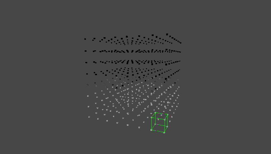
3D grid of weights used in marching cubes
0. Introduction
When developing a game we often require a landscape. This landscape can be created in many ways. The Unity game engine for example, has a built-in terrain system that allows us to raise and lower terrain, paint textures, place grass, etc. Unfortunately, this system comes with limitations, namely they do not support terrains with complex caves, ledges, and overhangs.
To solve this problem many game developers use an algorithm called ‘marching cubes’. This algorithm allows us to create 3D meshes that can be terraformed.
Popular games using similar techniques include No Man’s Sky, Astroneer, etc.
1. Understanding the algorithm
The marching cubes algorithm creates a polygonal surface mesh from a 3D scalar field by “marching” (looping) through the 3D space, and determining each configuration for the given cube.
Below you can see a simple visualisation. Every point in our 3D world is a value from 0 to 1, where 0 is black and above ground, and 1 is white and underground. We march a single cube through the 3D space and construct a mesh.
In practice, when creating a mesh we look at each possible cube in parallel rather than one cube at a time.
Note: In the downloads section, you can download this simple visualisation and its code (Unity3D, C#).
By looking at the values at the corners of a given cube, we can determine what the triangle configuration is for this cube.
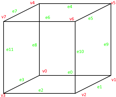
- Edge Index
- Vertex Index
When the value at a vertex is below a given threshold, also called isosurface, we can say that this vertex of our cube in the terrain is underground, so to speak. A configuration is than chosen by determining which of those vertices are below the isosurface, and which are not.
For example, if vertex 0 where to be of value -1.0, and all other vertices have a value of 1.0. Given that our isosurface is 0.5, we can conclude that since vertex 0 is the only vertex below the threshold, we want to hide this vertex by creating a triangle in front of it by connecting edges 0, 3 and 8.
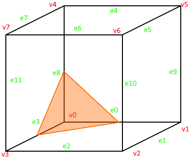
Configuration when only v0 is below threshold
In total there are 256 such combinations that can be formed by looking at the values of our vertices since cubes have 8 corners with each 2 possible states (28=256). These 256 configurations can be reduced to only 15, since most cases are symmetries. Luckly there are lookup tables for the configurations. We can find those on the internet, so we will be using one of those.
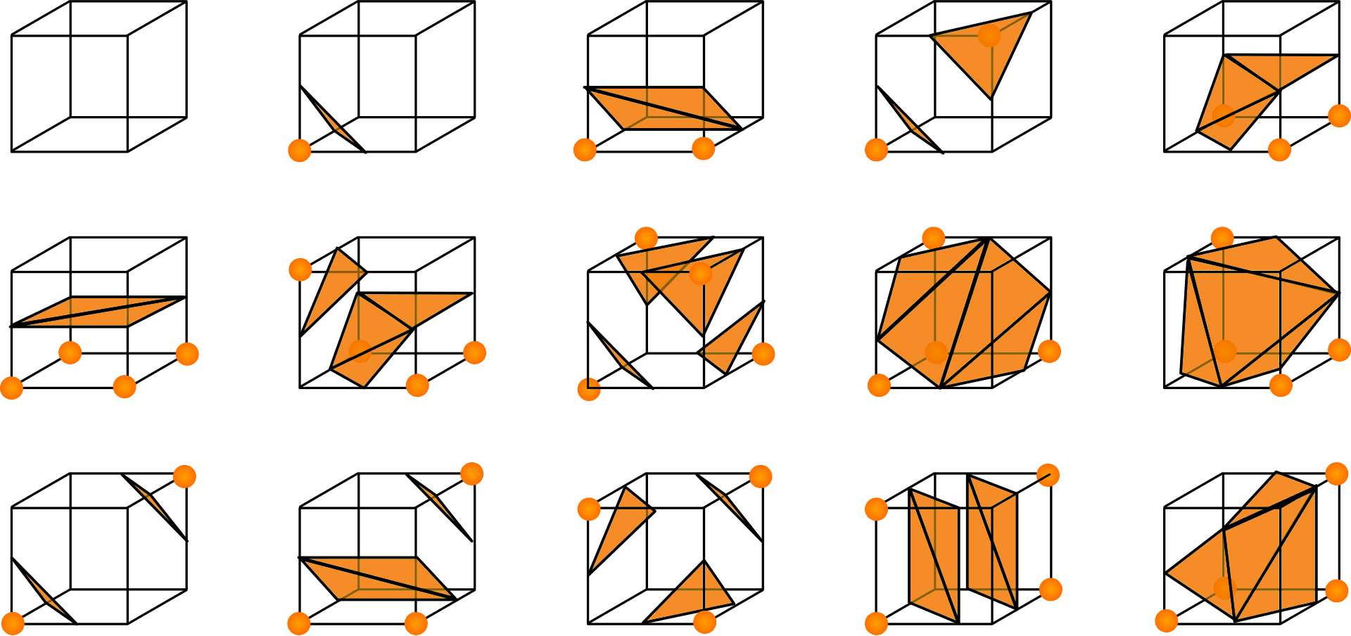
15 unique cases (source)
Once we have determined the configuration for a single cube and placed our triangles, we move on to the next and repeat the same process for all other cubes in the world.
2. The algorithm in code (HLSL)
Note: In the downloads section, you can download lookup tables
The algorithm begins by determining the configuration of the cube, by comparing the value of our cube at every corner vertex with the isosurface level.
1
2
3
4
5
6
7
8
9
int cubeIndex = 0;
if (cubeValues[0] < isolevel) cubeIndex |= 1;
if (cubeValues[1] < isolevel) cubeIndex |= 2;
if (cubeValues[2] < isolevel) cubeIndex |= 4;
if (cubeValues[3] < isolevel) cubeIndex |= 8;
if (cubeValues[4] < isolevel) cubeIndex |= 16;
if (cubeValues[5] < isolevel) cubeIndex |= 32;
if (cubeValues[6] < isolevel) cubeIndex |= 64;
if (cubeValues[7] < isolevel) cubeIndex |= 128;
Given our example above, where only vertex 0 was below the isosurface level, we will find that the configuration has an index of 1 (cubeIndex = 1).
Now that we have found what the configuration for the cube is, we want to know which the edges are that we have intersections with so that we can start adding triangles.
These edges can be found in a lookup table. The lookup table that we will use is the “triTable” (triangulation table)
1
int edges[] = triTable[cubeIndex];
Great, now we have our edges. Going back to our example above, we will find that the array of edges is filled with the following configuration
{0, 8, 3, -1, -1, -1, -1, -1, -1, -1, -1, -1, -1, -1, -1, -1}The way we have to read this array is quite simple, we look at 3 edge indices at a time, these edges will make up our triangle. Our first triangle is:
{0, 8, 3}The next edges however have values of -1, so we know these are not actually edges, since edges are between 0 and 7, and so we can stop creating triangles.
Now that we know the indices of the edges, we still have to find the 2 vertices that this edge is between. We do this by using another lookup table, “edgeConnections”. This table contains, given an edge index, the 2 vertices that this edge is between.
1
2
3
4
5
6
7
8
9
10
11
12
13
14
15
16
 for (int i = 0; edges[i] != -1; i += 3)
    {
        // First edge lies between vertex e00 and vertex e01
        int e00 = edgeConnections[edges[i]][0];
        int e01 = edgeConnections[edges[i]][1];

        // Second edge lies between vertex e10 and vertex e11
        int e10 = edgeConnections[edges[i + 1]][0];
        int e11 = edgeConnections[edges[i + 1]][1];

        // Third edge lies between vertex e20 and vertex e21
        int e20 = edgeConnections[edges[i + 2]][0];
        int e21 = edgeConnections[edges[i + 2]][1];

        // We add our triangle here
    }
Once again, looking at the example above, we know our edges are 0, 8, 3. Looking in the edgeConnections table, we will find that:
- edge 0 is between vertex 0 and vertex 1.
- edge 8 is between vertex 0 and vertex 4
- edge 3 is between vertex 3 and vertex 0
Up next, we can map those edge indices to an array containing our actual cube coordinates. Remember, these coordinates overlap with the following vertex positions:

static const float3 cornerOffsets[8] = {
		float3(0, 0, 1), // v0
		float3(1, 0, 1), // v1
		float3(1, 0, 0), // v2
		float3(0, 0, 0), // v3
		float3(0, 1, 1), // v4
		float3(1, 1, 1), // v5
		float3(1, 1, 0), // v6
		float3(0, 1, 0)  // v7
};
With this we know what the actual physical coordinates are of our cube vertices.
In the last step we have to interpolate between those found edges to estimate where along the edge the edge vertex actually is, this is done to give a smoother look. Interpolation can be done with the following formula.
1
2
3
4
float3 interp(float3 edgeVertex1, float valueAtVertex1, float3 edgeVertex2, float valueAtVertex2)
{
    return (edgeVertex1 + (isoLevel - valueAtVertex1) * (edgeVertex2 - edgeVertex1)  / (valueAtVertex2 - valueAtVertex1));
}
To wrap up, connect the edges, and add the triangle. We also can’t forget to adjust the actual global position of the cube, up to this point we have only been working with a local position where the xyz coordinates are all between 0 and 1. We obviously don’t want this to be local because all cubes would overlap which each other.
struct Triangle {
    float3 a, b, c;
};

AppendStructuredBuffer<Triangle> _Triangles;
1
2
3
4
5
6
7
8
9
10
11
12
13
14
15
16
17
18
19
20
21
22
for (int i = 0; edges[i] != -1; i += 3)
{
// First edge lies between vertex e00 and vertex e01
int e00 = edgeConnections[edges[i]][0];
int e01 = edgeConnections[edges[i]][1];
// Second edge lies between vertex e10 and vertex e11
int e10 = edgeConnections[edges[i + 1]][0];
int e11 = edgeConnections[edges[i + 1]][1];
// Third edge lies between vertex e20 and vertex e21
int e20 = edgeConnections[edges[i + 2]][0];
int e21 = edgeConnections[edges[i + 2]][1];
// worldPos is the coordinate (float3)
// of the cube itself in the game world.
Triangle tri;
tri.a = interp(cornerOffsets[e00], cubeValues[e00], cornerOffsets[e01], cubeValues[e01]) + worldPos;
tri.b = interp(cornerOffsets[e10], cubeValues[e10], cornerOffsets[e11], cubeValues[e11]) + worldPos;
tri.c = interp(cornerOffsets[e20], cubeValues[e20], cornerOffsets[e21], cubeValues[e21]) + worldPos;
triangles.Append(tri);
}
That seems to be it! In the next part of this series we will be taking the code written above and actually creating terrain in Unity3D.